Inference & Hypotheses
Skill Checklist
Track your progress across all skills in your objective. Mark your confidence level and identify areas to focus on.
Track your progress:
Don't know
Working on it
Confident
📖 = included in formula booklet • 🚫 = not in formula booklet
Track your progress:
Don't know
Working on it
Confident
📖 = included in formula booklet • 🚫 = not in formula booklet
Hypothesis Testing and p-values
Null and alternative hypotheses (H₀ & H₁)
The null hypothesis H0 states the baseline assumption, usually that no effect or relationship exists. If we reject the null hypothesis, we accept an alternative hypothesis H1.
Significance Levels & p-values
p-value: The probability of getting results as surprising (or more) as the observation if the null hypothesis were true.
Significance level (α): The cutoff we choose in advance. If the p-value is below α, we reject the null hypothesis.
χ² tests
Chi Squared (χ²) Goodness of Fit Test
A χ² goodness of fit test compares measured data to expected frequencies, and returns a p-value that captures the likelihood of equal or greater deviation from the expected frequencies. On a calculator:
Enter in L1 the observed frequencies
Enter in L2 the expected frequencies
Find the χ2 GOF-Test on your calculator, with
Observed: L1
Expected: L2
df: (n−1), where n is the number of items in either list
The calculator returns the p-value, which we interpret as usual for a hypothesis test. It also returns the value of χ2, which we can compare to a critical value if it is given.
Degrees of Freedom for a χ² goodness of fit test
When the total number of observations is fixed, and we have n different categories, we only have n−1 degrees of freedom since we can find one entry by subtracting the sum of the other entries from the total.
χ² critical value
The critical value for a χ² test is a threshold we are given, against which we compare the value of χ² for our data. If our χ² is larger than the critical value, we reject H0.
Chi Squared (χ²) Test For Independence
A χ2 test can also be used to test whether categorical variables are related, for example, does favorite movie depend on gender? It works by comparing how far off the observed data is from what we would expect if the variables were not related (H0).
On a calculator:
Enter the observed frequencies in a matrix (table)
Enter the expected frequencies in a separate matrix
Navigate to χ2-Test on your calculator, and enter the observed and expected matrices you just filled.
The calculator returns the χ2 value and the p value.
Further χ² tests & unbiased estimators
Grouping data for Chi squared (χ²) tests
Before performing a χ2 test, it's important to verify that all expected frequencies are larger than 5. If any are not, categories must be combined before performing the test. For example:
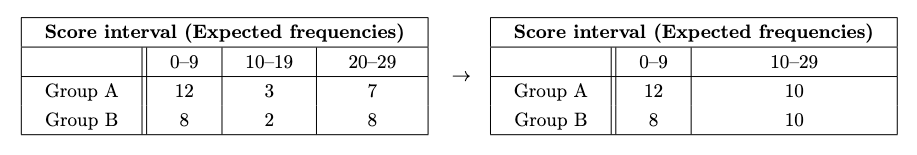
Note that when we combine categories, the degrees of freedom decrease!
x̅ as an unbiased estimate of μ
If the true mean of some distribution is unknown, we can average samples taken from the distribution to produce an unbiased estimate of the population mean:
We call the estimate unbiased since
sₙ₋₁² as an unbiased estimator of σ²
If the true variance of some distribution is unknown, we can use the sample standard deviation to get an unbiased estimate of the population variance:
(Your calculator returns both Sx - which is the same as sn−1 and σx).
We call the estimate unbiased since
Chi squared (χ²) with estimated parameters
When we perform a χ2 goodness of fit test with unbiased estimates as parameters for some distribution, each estimated parameter is an additional constraint on the data, so we need to subtract from the degrees of freedom:
where k is the number of parameters estimated.
Student's t-test
1 tailed and 2 tailed T-test hypotheses
Given a null hypothesis H0:μ=μ0, we can have any of the following alternative hypotheses
The first two alternative hypotheses are called one-tailed since we only care how far the sample mean, xˉ, is from μ0 in one direction. The last hypothesis is two-tailed because we care how far xˉ is from μ0 regardless of direction.
T-test for mean μ (1-sample)
We can perform a t-test for a single sample against a known mean by on a calculator:
Enter the sample data into a list.
Navigate to T-Test on a calculator.
Select "DATA" and enter the name of the list where sample is stored.
Select the tail type depending on what our alternative hypothesis is (μ0 is the population mean):
=μ0 for a change in mean
<μ0 for a decrease in mean
>μ0 for an increase in mean
Hit calculate, and interpret the p-value as usual.
2-sample T-Test
To compare the means of two samples using a T-test, we use a calculator:
Enter each sample in its own list.
Navigate to 2-SampTTest.
Select "Data", then enter the names of the lists containing the samples.
Select the tail type depending on what our alternative hypothesis is:
μ1=μ2 for different means
<μ2 for first list mean smaller than second
>μ2 for first list mean greater than second
Set "Pooled" to true.
The calculator reports the t-value and p-value, which we interpret as usual.
Paired tests for the mean
We say that data is paired when each value in one row is tied to the value in the next row. An example of this is before and after scores for a group of students.
Instead of comparing means using a two-sample test, we instead calculate the difference between the rows for each column, and then do a one-sample test with μ0=0.

Two important notes:
H0:d=0 and H1 can be d=0,d<0 or d>0.
The assumption being made is that the differences are normally distributed, not the original values.
Testing for population correlation: H₀ : ρ = 0 vs H₁ : ρ ≠ 0
We can test the correlation between two normally distributed populations.
Enter the samples into L1 and L2
Navigate to LinRegTTest.
Select ρ=0,<0 or >0
The calculator returns the p-value (not to be confused with ρ), as well as the coefficients y=a+bx.
Z-test and Confidence Intervals
Normal confidence interval using technology
Your calculator should include a statistical test called Zinterval or similar. To use it:
Enter the value of σ, which must be known for a Z-test of any kind.
Enter either
Data: a list of values you've typed into the calculator
Stats: the sample mean xˉ and n, the number of samples.
Enter the confidence level and hit calculate
The calculator returns the desired interval, which is symmetrical around xˉ.
T-interval confidence interval using technology
Your calculator should include a statistical test called Tinterval or similar. To use it:
Enter either
Data: a list of values you've typed into the calculator
Stats: the sample mean xˉ, the sample standard deviation Sx and n, the number of samples.
Enter the confidence level and hit calculate
The calculator returns the desired interval, which is symmetrical around xˉ.
Z-Test for population mean
Z-tests allow us to test the mean of a sample against
a population with known mean: use Z-Test
another sample: use 2-SampZTest
a paired sample: calculate the difference, then use Z-Test with μ0=0.
Critical values & regions
When testing the mean of a sample against a population, the critical region is the set of values for the sample mean that would lead to rejecting the null hypothesis. The critical value(s) is (are) the boundary of the critical region. In other words, the critical value is the threshold for xˉ that leads to a p value exactly equal to the chosen significance level.
Binomial & Poisson Tests
Binomial test for proportion
A binomial test for proportion checks whether the number of “successes” in a sample is consistent with a hypothesized population proportion p. To find the p-value, calculate the probability of observing results at least as extreme as your sample using the binomial distribution. On the calculator, use
bimomcdf(n,p,k−1) for P(X≤k) and
1−bimomcdf(n,p,k−1) for P(X≥k);
for a two-tailed test, double the smaller tail probability.
Poisson test for mean
A Poisson test for rate checks whether the number of observed events in a sample is consistent with a hypothesized mean rate λ. To find the p-value, calculate the probability of observing results at least as extreme as your sample using the Poisson distribution. On the calculator, use
poissoncdf(λ,k) for P(X≤k) and
1−poissoncdf(λ,k−1) for P(X≥k);
for a two-tailed test, double the smaller tail probability.