Differential Equations
Skill Checklist
Track your progress across all skills in your objective. Mark your confidence level and identify areas to focus on.
Track your progress:
Don't know
Working on it
Confident
📖 = included in formula booklet • 🚫 = not in formula booklet
Track your progress:
Don't know
Working on it
Confident
📖 = included in formula booklet • 🚫 = not in formula booklet
Solving Differential Equations
Separable Variables
When you have a differential equation in the form
you can bring all the y's to one side and all the x's to the other:
Particular Solutions
The solutions to differential equations will usually contain a constant of integration +C. These are called general solutions.
Often, we are given an initial condition, ie the value of y for a specific x, which we can use to solve for C. The result is the particular solution.
Euler's Method
Performing Euler's Method
Mathematically Euler's Method works as follows:
Start at a known point (x0,y0)
Pick a step size h such that x0+nh=xfinal for some integer n.
Repeat the following steps for each n until the desired x-value is reached:
Find the slope dxdy=f(xn,yn)
Find the next x value xn+1=xn+h📖.
Find the next y-value yn+1=yn+h×f(xn,yn)📖
Coupled systems
Coupled systems of differential equations
A system of differential equations is said to be coupled if the variables and their derivatives are interrelated, meaning knowledge of one variable depends on knowledge of another.
Coupled systems of differential equations can be written in the form
Euler's method for coupled systems
Let a coupled system of differential equations be given by the formulas
We can use Euler's method to find how the x and y values change when t moves in steps of size h by using the equations:
Finding eigenvector solutions of linear systems
If a coupled system of differential equations involves strictly linear equations of x and y, i.e. is of the form
for real numbers a,b,c, and d, then the system can be written in matrix form as
If M has real and distinct eigenvalues λ1 and λ2 that produce the corresponding eigenvectors p1 and p2, the general solution of the system is given by
Stable, unstable and saddle points
If as t increases the solution curves move
all towards the equilibrium point, then the point is stable
all away from the equilibrium point, then the point is unstable
some towards and some away from the equilibrium point, then the point is a saddle point
Phase portraits for real distinct eigenvalues
For a coupled system whose matrix M has real and distinct eigenvalues, the phase portrait will have stream lines that approach the direction of the eigenvector with the larger eigenvalue. The process for sketching is as follows:
Draw the eigenvectors as straight lines through the origin (or other equilibrium point)
Consider which case the eigenvalues satisfy:
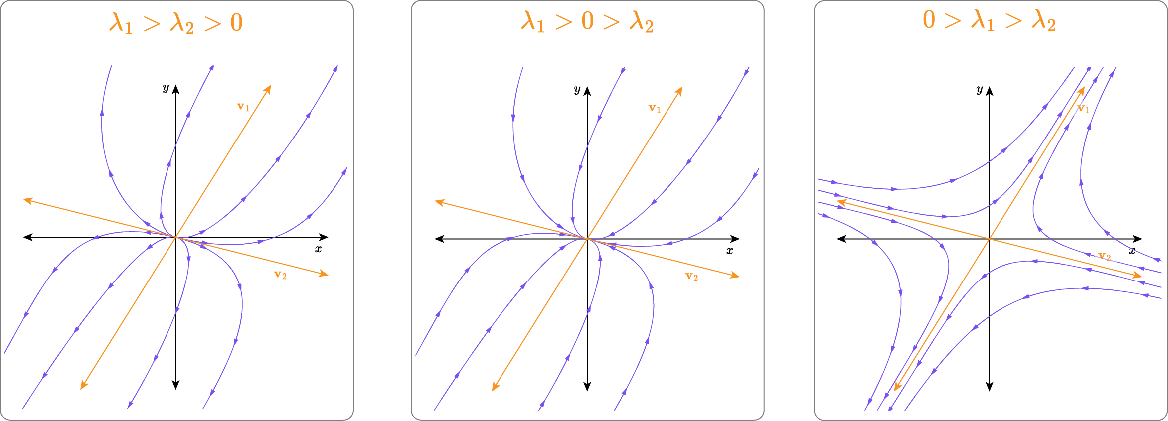
The sign of the eigenvalues determines whether we have an unstable node, stable node or saddle point.
The solution curves start in the direction of v2, the eigenvector with the smaller eigenvalue, and end in the direction of v1 with the larger eigenvalue.
Draw at least one solution curve in each quadrant generated by the intersecting eigenvectors.
Phase portraits for complex eigenvalues
When the eigenvalues of a coupled system are complex, say
the solution curves follow 3 possible shapes in a phase portrait:
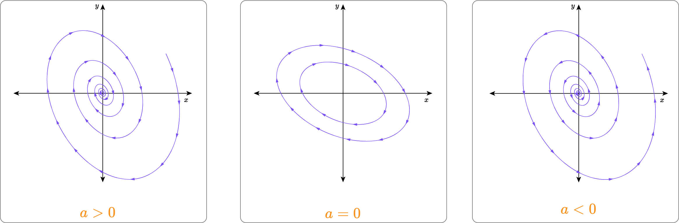
a>0: an unstable spiral,
a=0: an ellipse,
a<0: a stable spiral.
Once the shape is known, we can determine whether the trajectories are clockwise or counterclockwise by evaluating dtdx at (0,1):
dtdx<0, spiral is counterclockwise
dtdx<0. spiral is clockwise
This is equivalent to looking at the top right of the matrix:
Second Order Differential Equations
Second order differential equations
A second order differential equation is a differential equation of the form
To solve these equations, we rewrite it as a system of coupled first order equations. Using the fact that dtd2x=dtd(dtdx) and substituting dtdx=y,
This equation can be solved with the usual techniques for coupled systems. On exams, questions involving second-order differential equations are usually set in a real-world context such as movement.