Topics
Skill Checklist
Track your progress across all skills in your objective. Mark your confidence level and identify areas to focus on.
23 Skills Available
Track your progress:
Don't know
Working on it
Confident
📖 = included in formula booklet • 🚫 = not in formula booklet
Track your progress:
Don't know
Working on it
Confident
📖 = included in formula booklet • 🚫 = not in formula booklet
Hypothesis Testing and p-values
2 skills
Null and alternative hypotheses (H₀ & H₁)
SL AI 4.11
When we want to make a claim using statistics, need sufficient evidence. Flipping a coin and getting 3 heads in a row is not strong evidence that it is biased, but 100 in a row is.
Whatever data we have, we start by assuming that they are produced by random chance alone. We call this the null hypothesis, which we write H0. In the coin flip example, the null hypothesis is H0: the coin is fair.
An alternative hypothesis, denoted H1, is the idea that something "fishy" is going on. In the coin flip example, this could be H1: the coin is biased towards heads.
It's important (both in exams and real life) to assume the null hypothesis is true unless you have good evidence.
Writing down the null and alternative hypotheses can be hard, but you can think of H0 as a neutral assumption, and H1 as something we need evidence to prove.
More Examples
Does listening to music while studying hurt test performance?
Null hypothesis H0: we assume it makes no difference: the average scores of students with or without music are similar
Alternative hypothesis H1: students who listen to music do worse: they have a lower average test score.
Does drinking an energy drink improve reaction time?
Null hypothesis H0: we assume it makes no difference: the average reaction times with and without energy drinks are similar.
Alternative hypothesis H1: drinking an energy drink lowers the mean reaction time.
Significance Levels & p-values
SL AI 4.11
Once we have our null and alternative hypotheses, we use our data as evidence against the null hypothesis.
Let's take the coin flip example, and start by assuming the null hypothesis: it is fair. That means each time I flip it, I have a 21 probability of getting heads. If the coin gives 10 heads in a row, the probability is
(21)10≈0.098%
This number is the probability of the data we observed assuming the null hypothesis. The smaller it gets, the less likely that the null hypothesis is true.
We call this the p-value. The smaller the p-value, the stronger the evidence for the alternative hypothesis. If the p value is less than the significance level α, we reject the null hypothesis, which is essentially concluding the alternative hypothesis is true.
p-value: The probability of getting results as surprising (or more) as the observation if the null hypothesis were true.
Significance level (α): The cutoff we choose in advance. If the p-value is below α, we reject the null hypothesis.
χ² tests
4 skills
Chi Squared (χ²) Goodness of Fit Test
SL AI 4.11
A χ² goodness of fit test compares actual frequencies to the frequencies that would be expected under the null hypothesis. The bigger the relative difference between actual and expected values, the smaller the p value it returns.
For example, imagine a 5 kilometer race where the number of racers finishing in certain time brackets is recorded, and compared to what is expected based on historical data:
Notice that the expected and observed frequencies both add up to 146. They must always be the same.
The null hypothesis for this test is that the observed frequencies do fit the expected distribution.
The alternative hypothesis is that the observed frequencies do not fit the expected distribution.
To perform a χ² goodness of fit test, you use your calculator:
Enter in L1 the observed frequencies
Enter in L2 the expected frequencies
Find the χ2 GOF-Test on your calculator, with
Observed: L1
Expected: L2
df: (n−1), where n is the number of categories. (2 in our case)
The calculator returns the following:
χ2≈9.24
p≈0.00986
Degrees of Freedom for a χ² goodness of fit test
SL AI 4.11
The degrees of freedom in a dataset is the number of values that can change while keeping the total sum constant. If there are n values in a list, the number of degrees of freedom is n−1.
The degrees of freedom are important because with more values, there will naturally be more total variation between actual and expected values. The calculator needs to account for this.
χ² critical value
SL AI 4.11
The critical value for a χ² test is a threshold we are given, against which we compare the value of χ² for our data. If our χ² is larger than the critical value, we reject H0.
Chi Squared (χ²) Test For Independence using technology
SL AI 4.11
A χ2 test can also be used to test whether categorical variables are related, for example, does favorite movie depend on gender? It works by comparing how far off the observed data is from what we would expect if the variables were not related (H0).
In a χ2 test for independence:
The null hypothesis H0 is that the categories are not independent (not related)
The alternative hypothesis H1 is that the categories are not independent (they are related).
On a calculator:
Enter the observed frequencies in a matrix (table)
Enter the expected frequencies in a separate matrix or leave them blank if they are not given.
Navigate to χ2-Test on your calculator, and enter the observed and expected matrices (select an empty matrix and your calculator will find the expected values itself) you just filled.
The calculator returns the χ2 value and the p value.
Student's t-test
4 skills
1 tailed and 2 tailed T-tests and their hypotheses
SL AI 4.11
A T-test is a technique that compares whether the means of two groups are significantly different. It works by measuring how different the mean of a sample is from another mean, and comparing that difference to the variance in the sample.
The null hypothesis is that the two groups have the same mean H0:μ=μ0.
We can have any of the following alternative hypotheses:
H1:μ<μ0 - testing whether our sample has a lower mean that what we're comparing it to
H1:μ>μ0 - testing whether our sample has a higher mean that what we're comparing it to
H1:μ=μ0 - testing whether our sample has a different mean that what we're comparing it to
The first two alternative hypotheses are called one-tailed because they test difference in a specific direction (one mean greater or smaller than the other).
Examples
We can use a one-tailed T-test to determine whether
patients at a certain hospital have a significantly faster (lower) mean recovery time than the national average. This is a one-tailed test.
trout in lake A have a significantly different mean weight than trout in lake B. This is a two-tailed test.
T-test for mean μ (1-sample)
SL AI 4.11
We can perform a t-test for a single sample against a known mean by on a calculator:
Enter the sample data into a list.
Navigate to T-Test on a calculator.
Select "DATA" and enter the name of the list where sample is stored.
Select the tail type depending on what our alternative hypothesis is (μ0 is the population mean):
=μ0 for a change in mean
<μ0 for a decrease in mean
>μ0 for an increase in mean
Hit calculate, and interpret the p-value as usual.
Assumptions: This test is assuming that the data are independent, randomly sampled, and approximately normally distributed. IB questions will specifically ask you to state the assumption of normally distributed variables.
2-sample T-Test
SL AI 4.11
To compare the means of two samples using a T-test, we use a calculator:
Enter each sample in its own list.
Navigate to 2-SampTTest.
Select "Data", then enter the names of the lists containing the samples.
Select the tail type depending on what our alternative hypothesis is:
μ1=μ2 for different means
<μ2 for first list mean smaller than second
>μ2 for first list mean greater than second
Set "Pooled" to true.
The calculator reports the t-value and p-value, which we interpret as usual.
Assumptions: This test is assuming that the data are approximately normally distributed, and that both samples have the same variance. IB questions will specifically ask you to state these assumptions.
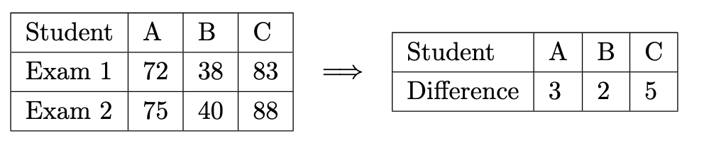
Paired tests for the mean
AHL AI 4.18
We say that data is paired when each value in one row is tied to the value in the next row. An example of this is before and after scores for a group of students.
Instead of comparing means using a two-sample test, we instead calculate the difference between the rows for each column, and then use a 1 sample T test with μ0=0.
Two important notes:
H0:d=0 and H1 can be d=0,d<0 or d>0.
The assumption being made is that the differences are normally distributed, not the original values.
Z-test and Confidence Intervals
5 skills
Understanding confidence intervals
AHL AI 4.16
A confidence interval is a range of values in which we believe the true mean of the population lies.
When we take samples from a larger population, our samples tend to cluster around the mean of the population. Using a sample, we can make an educated guess that the true population mean is in some range. The more data we have, the better our guess gets.
We calculate this interval in line with the level of certainty we want to have that our range contains the true mean. Obviously, we can be 100% sure that the value is between −∞ and +∞, but the smaller the range, the lower the confidence level we can have.
Normal confidence interval using technology
AHL AI 4.16
If we know the standard deviation of the population whose mean μ we want a confidence interval for, we use a so called normal confidence interval.
Your calculator should include a statistical test called Zinterval or similar. To use it:
Enter the value of σ, which must be known for a Z-test of any kind.
Enter either
Data: a list of values you've typed into the calculator
Stats: the sample mean xˉ and n, the number of samples.
Enter the confidence level and hit calculate
The calculator returns the desired interval, which is symmetrical around xˉ.
T-interval confidence interval using technology
AHL AI 4.16
To find a confidence interval for the mean without knowing the variance, we first have to use our sample to first estimate the standard deviation. Because of this extra uncertainty, we switch to using a t-distribution.
Your calculator should include a statistical test called Tinterval or similar. To use it:
Enter either
Data: a list of values you've typed into the calculator
Stats: the sample mean xˉ, the sample standard deviation Sx and n, the number of samples.
Enter the confidence level and hit calculate
The calculator returns the desired interval, which is symmetrical around xˉ.
Z-Test for population mean
AHL AI 4.18
Z-tests allow us to test the mean of a sample against
a population with known mean: use Z-Test
another sample: use 2-SampZTest
a paired sample: calculate the difference, then use Z-Test with μ0=0.
Critical values & regions
AHL AI 4.18
When testing the mean of a sample against a population, the critical region is the set of values for the sample mean that would lead to rejecting the null hypothesis. The critical value(s) is (are) the boundary of the critical region. In other words, the critical value is the threshold for xˉ that leads to a p value exactly equal to the chosen significance level.
Further χ² tests & unbiased estimators
4 skills
Grouping data for Chi squared (χ²) tests
AHL AI 4.12
Before performing a χ2 test, it's important to verify that all expected frequencies are larger than 5. If any are not, categories must be combined before performing the test. For example:
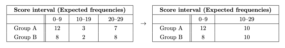
Note that when we combine categories, the degrees of freedom decrease!
x̅ as an unbiased estimate of μ
AHL AI 4.14
If the true mean of some distribution is unknown, we can average samples taken from the distribution to produce an unbiased estimate of the population mean:
μ≈xˉ=n∑xi.
We call the estimate unbiased since
μ=xˉ as n→∞
sₙ₋₁² as an unbiased estimator of σ²
AHL AI 4.14
If the true variance of some distribution is unknown, we can use the sample standard deviation to get an unbiased estimate of the population variance:
σ2≈Sx2=sn−12=n−1nσx2
(Your calculator returns both Sx - which is the same as sn−1 and σx).
We call the estimate unbiased since
σ2=Sx2 as n→∞
Chi squared (χ²) with estimated parameters
AHL AI 4.12
When we perform a χ2 goodness of fit test with unbiased estimates as parameters for some distribution, each estimated parameter is an additional constraint on the data, so we need to subtract from the degrees of freedom:
df =n−1−k
where k is the number of parameters estimated.
Testing for correlation ρ
2 skills
Bivariate normal distribution
AHL AI 4.18
A bivariate normal distribution is a two dimension distribution of points (x,y) where the data clusters around center point and spreads out like a normal distribution in every direction.
Testing for population correlation: H₀ : ρ = 0 vs H₁ : ρ ≠ 0
AHL AI 4.18
We can test the significance of a correlation between two variables using a special kind of T-test.
To perform this test, it must be known or assumed that the data points (x,y) follow a bivariate normal distribution.
Enter the samples into L1 and L2
Navigate to LinRegTTest.
Select ρ=0,<0 or >0
The calculator returns the p-value (not to be confused with ρ), as well as the coefficients y=a+bx.
To understand what this does, consider the following two graphs:
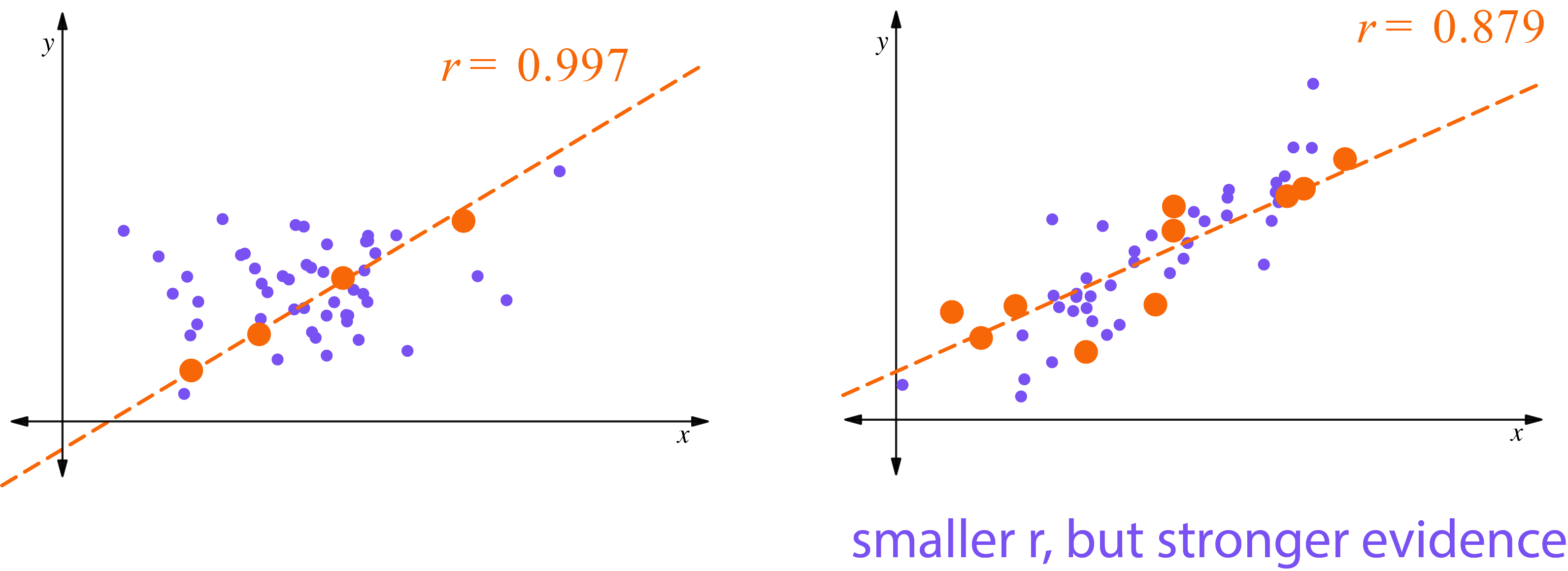
The graph on the left illustrates how a small sample of points can appear highly correlated even if the broader points are not. A larger sample of points showing a correlation is stronger evidence for the underlying correlation.
Binomial and Poisson Tests
2 skills
Binomial test for proportion
AHL AI 4.18
A binomial test for proportion checks whether the number of “successes” in a sample is consistent with a hypothesized population proportion p.
To find the p-value, calculate the probability of observing results at least as extreme as your sample using the binomial distribution. On the calculator, use
bimomcdf(n,p,k−1) for P(X≤k) and
1−bimomcdf(n,p,k−1) for P(X≥k);
Warning: it's easy to mix up the p value and the binomial probability p.
Note: The syllabus guide explicitly notes that only one-tailed Binomial tests will be required.
Poisson test for mean
AHL AI 4.18
A Poisson test for rate checks whether the number of observed events in a sample is consistent with a hypothesized mean rate λ.
To find the p-value, calculate the probability of observing results at least as extreme as your sample using the Poisson distribution. On the calculator, use
poissoncdf(λ,k) for P(X≤k) and
1−poissoncdf(λ,k−1) for P(X≥k);
Note: The syllabus guide explicitly notes that only one-tailed Poisson tests will be required.